Tables and Visual descriptors in MS Excel
In this post I am going to show you how you insert Tables and visual descriptors in Microsoft Excel. The post includes counting the records and five basic mathematical operations such as addition, subtraction, multiplication, division and averaging. If you do not read the fifth post , I recommend you to read I recommend you to read the following posts related to Microsoft excel.
- Basic Guide of Microsoft excel.
- Start with Microsoft excel.
- Font formatting in Microsoft excel document.
- Microsoft Excel sheet manipulation.
- Mathematical operations of Excel.
You can get the Microsoft excel application from Get into PC.
Tables and Visual descriptors in MS Excel (Insert tables)
You can insert table in excel document. Follow the following steps.
Steps
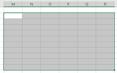
- Select the rows and columns.
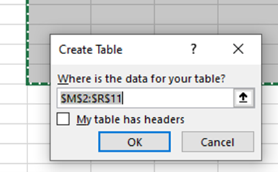
2. Click on insert menu. You will get the following option window that shows the starting cell and ending cell where the table will cover.
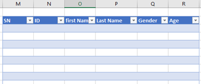
3. Click on Ok button. You will get the following result.
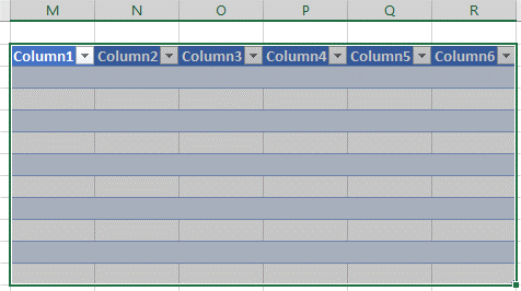
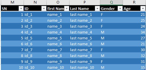
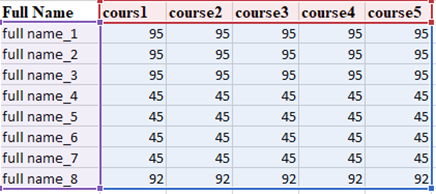
4. You can click on each column and give the field name for each column as follows.
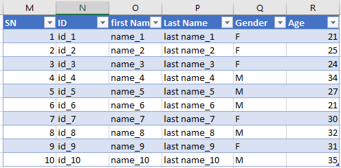
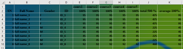
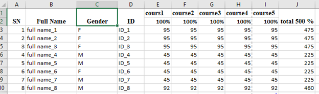
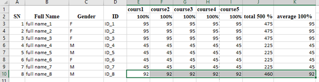
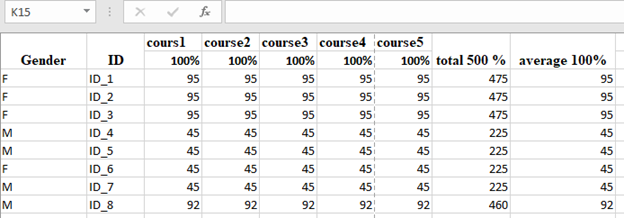
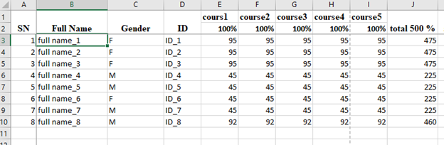
5. You can enter the data inside the inserted table as follows
Formatting tables
You can change the appearance and style of tables inside excel document.
Steps
- Select the table you want to change its format.
2. Click on home menu.
3. Go to style tool.
4. Click on the down arrow of format as table.
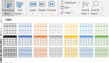
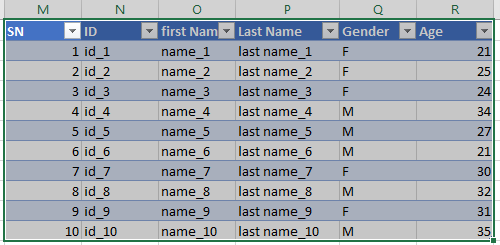
5. Select a table style you want to change. You will get the following result.
Tables and visual descriptors in MS excel (Insert Illustration)
If necessary, you can add the following illustrations in excel document.
- Shapes
- Pictures
- Icons
- Smart arts and 3D shapes
The steps you can follow is the same for all illustrations.
Insert pictures
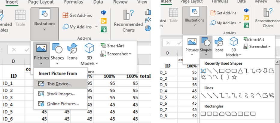
- Click on insert menu.
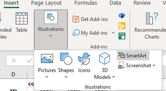
- Click on the down arrow of illustration button.
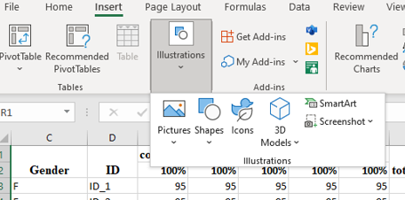
3. Select the illustration type. E.g., you may want to insert shapes and pictures as follows. The picture source may be local storage, picture from stocks or other online sources.
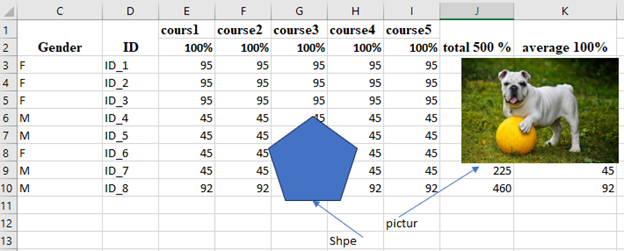
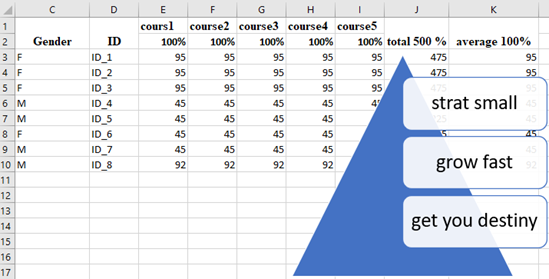
4. When you apply the above picture and shape inserting activity, you will get the result like the following excel sheet.
Insert smart arts
You can use the above procedure of picture and shape insertion.
The result will be as follows.
Tables and Visual descriptors in MS Excel (Insert Add-ins)
Excel application has two add-in tools. Thus, are Get Add-in and My Add-in.
Get Add-ins
You can find add-in that add new functionality to Office excel to simplify tasks and connect you to online services you use every day activity.
My Add-ins
You can insert the add-in in excel and use the web to enhance your activity.
Steps
- Click on insert menu.
- Got to add-ins tool.
- Click on get Add-ins or on My Add-ins as follows.
Insert Charts
You may want to do some data analysis from excel document using charts. So, you may use different charts according to the type of data you are going to make analysis. The common types of charts are.
- Bar chart
- Line chart
- Pi chart
- Scatter cart
- Statistic chart and many other.
To use the above charts, use the following steps.
- Select the records in the excel document you want to make data analysis.
2. Click on insert menu.
3. Go to charts tool.
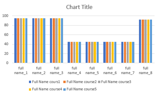
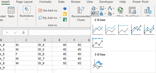
4. Select the type of charts you want to use.
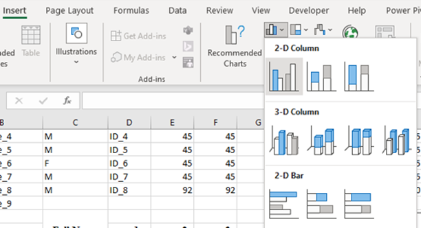
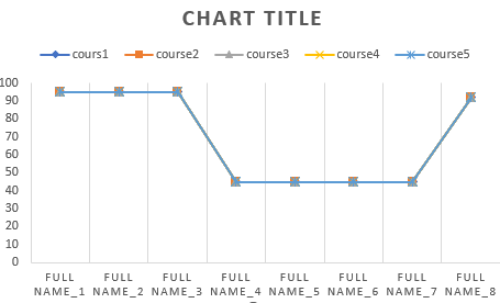
5. The result will be as follows. You can edit the chart title by your own name.
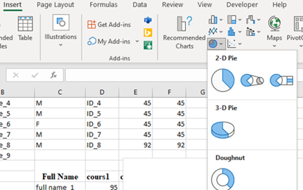
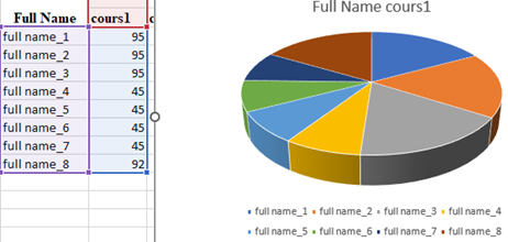
Use pi chart if the records have one column data.
You may also use 2-D line chart as follows.
Background image of MS excel sheet
You can insert background image of excel using the following procedure.
Steps
- Click on page layout menu.
- Go to page setup.
- Click on background. You will get the following option. Either you can insert background image from the internet or from local file storage. To insert from local file, click on work offline option.
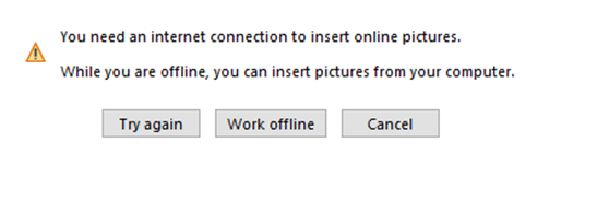
4. When you click on work offline option the following file selection window will appear.
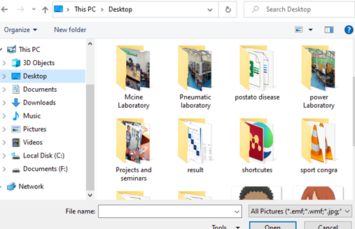
Select the background image and click on ok button. You can get the following result.
Get and transform data
You can import CSV data, Data from Database, data from website and data from local file.
Steps
- Click on data menu.
- Go to get and transform data tool.
- Click on the type of sources you are going to import external data.
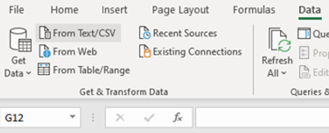
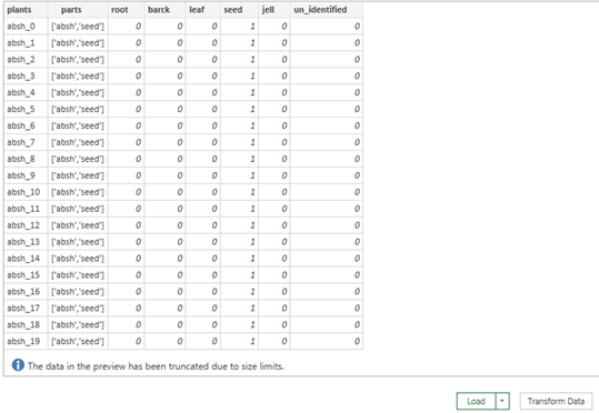
4. The following file selection window will appear. Because you select the data source from Text/CSV.
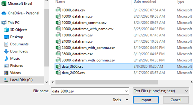
5. Select the data and click on import button. The following window will appear. To finalize data importing task, click on load button.
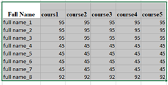
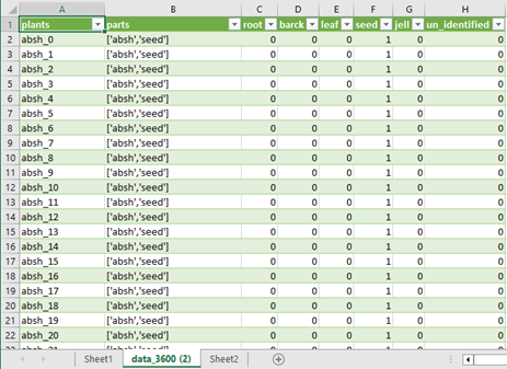
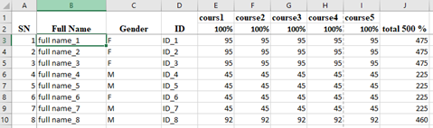
6.The imported data will look like the following excel sheet.
Thesaurus
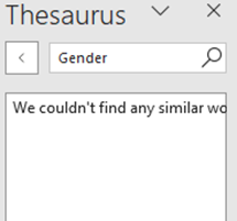
Thesaurus enables you to find the synonymous meaning of a words or phrases in the cells.
Steps
- Select the word or phrase in a cell.
2. Click on review menu.
3. Go to proofing tool.
4. Click on thesaurus.
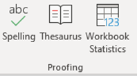
5. The result will be as follows.
Workbook statistics
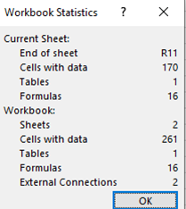
Using workbook statistics, you can get knowledge about how many cells, rows, columns, formulas, charts, tables and other contents present in your excel document.
Steps
- Click on review menu.
- Click on workbook statistics.
- You will get the result looks like the following information.
Tables and Visual descriptors in MS Excel (Comments)
You can give comments for a given cells, columns, rows or the whole records in excel file.
Steps
- Select the cell, rows, columns, or records you want to give a comment.
2. Click on review menu.
3. Go to comments tool.
4. Click on comment.
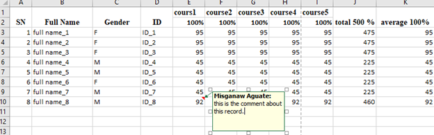
To delete the comment, click on the cell that has triangular red color at the right top corner. Then click on delete comment.
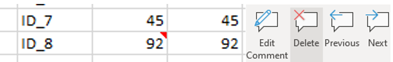
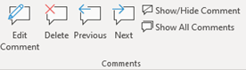
To show or hide the comments in excel, click on Show / Hide comments button found at comments tool.
Protect workbook
Keep other users making structural change to your workbook, such as moving, adding or deleting sheets.
Steps
- Click on review menu.
- Go to protect tool.
- Click on protect workbook. You will get the window option that request you to enter protection password.
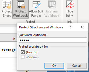
4. Enter the protection password and click Ok button. The excel again request you to enter the conformation password.
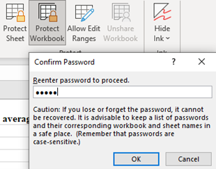
5. Finally, your workbook will protect from unauthorized user.
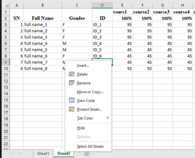
Tables and Visual descriptors in MS Excel (Protected workbook)
As shown in the following snapshot, delete, rename, move or copy, insert and other option are inactive. These options are disabled unless you unprotected the workbook by providing the password.
The following snapshot shows you the difference between protected workbook and unprotected workbook.
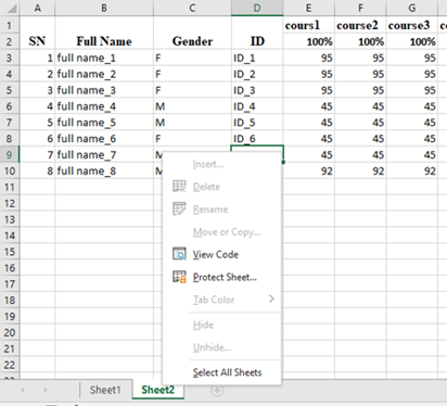
When you enter the password and unprotected the workbook, all the above option will be active. That means you can insert, add, rename, copy or edit the sheets.
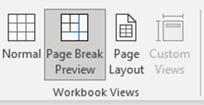
Workbook view
You can view your worksheet in normal view, page break preview and page layout view. Using page break preview, you can able to see where the page break will appear when the worksheet is printed. Using page layout, you can see how your printed document look like.
Steps
- Click on view menu.
- Go to workbook views
- You can click on page break preview to see to see where the page break is appeared for printing.
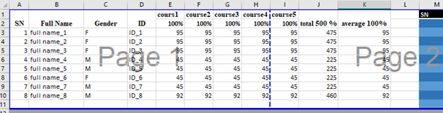
4. You can also click on page layout to how excel file will look when printed.
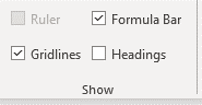
Hide and show grid lines
You can hide and show grid lines, headers and formula bar of excel file.
Steps
- Click on view menu.
- Go to show tool.
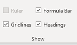
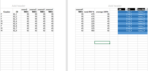
3. Check and uncheck the check box of grid lines. When you make uncheck, you will get the following result.
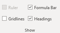
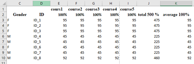
4. Check and uncheck the check box of header. when you uncheck the headings, the row labels 1, 2, 3, …. And the column heading A, B, C, … will be disappeared. As follows.
Tables and Visual descriptors in MS Excel (Freeze Panes)
Makes some portion of the sheet visible while you scroll through the rest of the sheet.
Steps
- Select the intersection cell of rows and column of the sheet to freeze both row and column. The following cell is selected to freeze the first column and row.
2. Click on view menu.
3. Go to window tool.
4. Click on freeze panes.
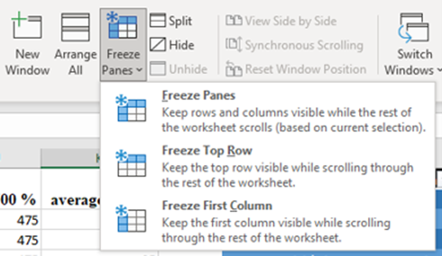
5. As shown in the above snapshot, you can freeze only columns, only rows or all rows and columns. If you are able to identify, the frozen row and column has thick line.
Thank you for reading.!!!! For more information about our service visit this site.