Microsoft Excel Sheet Manipulation

In this post I am going to show you Microsoft Excel sheet manipulation in Microsoft excel. The post includes insert different contents in MS excel. If you do not read the third post , I recommend you to read I recommend you to read the following posts related to Microsoft excel.

• Basic Guide of Microsoft excel.
• Start with Microsoft excel.
• Font formatting in Microsoft excel document.

You can get the Microsoft excel application from its official site.

Microsoft Excel sheet manipulation (Insert columns and rows)

You can insert excel sheet column or rows in the following way

• In between two rows or two columns.
• At the top (beginning) of the row record.
• At the left side (beginning) of the column record.

Insert columns

1. Hover the mouse cursor on the letter that represents the column.
2. The black down arrow will come. Then click to select the entire sheet column

3. Go to cells tool.

4. Click on the down arrow of insert button. You will get the following option window.

5. If your intention is inserting new row, click on insert sheet rows. If your goal is inserting column, click on insert sheet columns

Example 1: insert column between two columns

Let you take the above excel sheet, and you want to add (insert) service year column between Gender and salary column. The result will be the following excel sheet.

Select the sheet column. The new column is always inserted to the left side of the select column. In the following excel sheet, the service year is added from the left side of the selected column (salary).

Insert rows

Let you take the above excel sheet, and you want to add (insert) one record between Tigst and sable rows. The result will be the following excel sheet. What you should do is, hover the mouse cursor on row 9 and click on it to select the sheet row of row 9.

Let you want to add one record called record of TEBABLE ALEMU WRKQNEH, age = 45, service year = 30, Gender = Male, salary = 45,000.00, performance = 0.95123.

Microsoft Excel sheet manipulation (Deleting column and row)

Deleting column

In excel sheet, there may be unnecessary rows or columns after some day. Hence, you can remove the rows and columns using the following steps.

Steps

1. Select the rows or columns you want to delete. E.g., You want to remove service year column.

2. Click on home menu.

3. Go to cells tool.

4. Click on the down arrow under the delete button.

5. If you want to remove rows, click on delete sheet rows otherwise if the target is removing columns, click on delete sheet columns.

The result will look like as follows. After selecting the service year column and clicking the delete sheet columns button, the column service year is removed.

Deleting excel sheet rows

Deleting rows has the same procedure with removing column. The only difference is, selecting the required rows and click on delete sheet rows.

Example: deleting rows

If you want to delete the record of Row 9 (TEBABEL). Select the row TABABEL, go to Delete and click on delete sheer rows ended.

The result will be as follows. The record TEBABEL is removed.

Microsoft Excel sheet manipulation (excel sheet formatting)

This tool is used to do the following activities.

• Change the row height and column width.
• Organize sheets.
• Protect (lock) excel cell or excel sheet.
• Hide and unhide rows or columns and any more.

Change spaces of rows and columns

Steps

1. Select he rows or columns you want to increase or shrink the space.

2. Click on home menu.

3. Go to cells tool.

4. Click on the down arrow of format button. The following option window will appear.

5. If you want to change the width of column, click on column width. If your target is changing row height, click on rows height.

6. When clicking on column width you will get the following attempt window. Enter the value of column width and click on Ok button.

Example 1: change the width of the column

Let you want to change the column width of performance is 30. You will get result as follows.

Example 2: change the height of the rows

Let you want to change the row width of the first record is 30. You will get result as follows.

Hide and unhide rows and columns

There may be columns or rows to be hidden for some reason. So, hide and unhide tool helps you to do these activities.

Hide columns or rows

Steps

1. Select the columns or rows you want to hide.
2. Click on home menu.
3. Go to cells tool.
4. Click on the down arrow of format table.
5. Go to visibility option and hover on it.
6. Then click hide rows or columns. Another time, you can unhide the hidden rows or columns.

Example

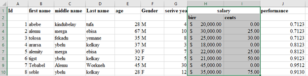
Let you want to hide the salary column of the following excel sheet.

The vertical green line shows there is hidden column between service year and performance column.

Unhide columns and rows

If there is a hidden column or rows, you can return back to its visibility status.

Steps

The procedure for unhiding is the same as hiding.  The difference is instead of clicking on hiding you will click on unhide rows or column button.

Example

The following excel sheet shows the hidden salary column is unhide (return back to its visibility status).

Microsoft excel sheet manipulation (Protecting sheet)

Prevent any change on the excel sheet from others user by limiting them the ability to edit cells, columns, or rows data.

Steps

1. Click on home menu.
2. Go to cells tool and click on the down arrow of format button.
3. From the format option, click on protect sheet as follows.

When clicking on protect sheet, the following option will appear. Give password that will not be accessible by other users except admin. For example, another user is permitted to select locked cell and select unlocked cell. Other operations are not allowed. When you complete assigning access permission, click on ok button.

After making the sheet protected, it will show the following message while you want to try access each cell.

If you are administrator or authorized user, you can follow the following procedure and unlock the excel sheet.

1. Click on home menu.
2. Go to cells tool and click on the down arrow of format button.
3. Click on unprotect sheet.

4. When you click on unprotect sheet, the excel request you to enter the password by which the sheet is protected.

Microsoft excel sheet manipulation (Sort and filter)

Sort data

Used to organize the data in the way that the data will be easily analyze. Mostly we sort and filter the excel data using its column.

Steps

1. Select the single column or the whole records.
2. Selecting single column to be sorted.

2. or Select records to be sorted.

3. Click on home menu.

4. Go to editing.

5. Clock on the down arrow of sort and filter button.

6. Select smallest to largest or A to Z for ascending order. Select sort largest to smaller or Z to A for descending order. In the following excel sheet, the record is sorted in ascending order.

Filter data

You can filter the record in excel sheet using the specific columns. Using specific columns, you can filter the data you want to display. E.g., You may want to filter the data using ID in the above excel sheet.

Steps

The procedure to filter data is the same as sorting data. In data filtering, you will click on filter option.

While clicking on filter option, the excel sheet will look like as follows.

E.g., You want to filter the data by gender column and display only the record assigned by M, hence you will uncheck the F check box and click on Ok button or press enter key from the keyboard. The result will be all records labeled by M will be displayed.

The above excel sheet is the result of filtered data using Gender column. Hence, the sheet only shows the records with gender of M. To return back to show both M and F, click on the down arrow of Gender column with the filtration icon.

Click on the uncheck checkbox of F to display records labeled with gender F and click on OK button or press enter key from the keyboard.

Remove filter icon from Microsoft excel sheet column header

When you apply filtration, there is filter icon at the right side of each column header. The down arrow sign at each column is called filtration icon. The following procedure help you to remove this icon from each column header.

1. Go to the sort & filter tool.
2. Click on filter.

3. The icon will be removed from the columns.