Mathematical operations of Microsoft Excel

In this post I am going to show you Mathematical operations of Microsoft Excel. The post includes counting the records and five basic mathematical operations such as addition, subtraction, multiplication, division and averaging. If you do not read the forth post , I recommend you to read I recommend you to read the following posts related to Microsoft excel.

• Basic Guide of Microsoft excel.
• Start with Microsoft excel.
• Font formatting in Microsoft excel document.
• Microsoft Excel sheet manipulation.

You can get the Microsoft excel application from its official site.

Mathematical operations of Microsoft Excel (Auto SUM)

You can calculate the sum, average, count, maximum and minimum value of a given selected column or rows. The result will appear after the selected cell.

steps

1. Select the columns or rows to calculate its sum, average, min, maximum or other calculation.

1. Click on home menu.
2. Go to editing tool.
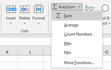
3. Click on the down arrow of auto sum.
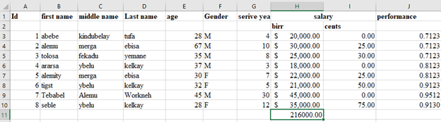
4. Click on the option you want. E.g., you may select sum to calculate the total salary in the following excel sheet.

Example 1: Sum of salary

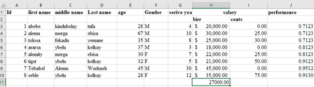
Example 2: average salary

Mathematical operations in Microsoft excel (Count records)

You can count records to know how many records present in you excel sheet. You may count the following type of record.

• Simply rows
• Gender to know total female and male.
• Number of records that has something greater or less than a given values.

Count number of records or rows

Steps

1. Select the cell where you want to put the result of count.

1. Write the following formula inside the selected count.

=COUNT (A3:A10)

Where A1 is a row 1 in A column where count is started. A10 is the last row where count is completed.

• Then you can get the following result.

Count the total MALE and FEMALE in excel sheet.

Steps

1. Select the cell where you want to write the result of count.

2. Write the following formula in the selected cell.

To count the number of MALE,

= COUNTIF (starting row Colum: ending column row,” M”)

Remember, you have to specify the column where the gender is present. E.g., in the following excel sheet, the gender is found at F column.

3. After writing the formula press enter key from the keyboard.

Based on the above formula, you will get the following result.

Single count function

You may want to count how many records is present that has the value greater than or less than a given range.

Steps

1. Select the cell where you want to write the result of count.
2. Write one of the following formulas inside a selected cell as your need.
3. = COUNTIF (column row: column row,”> some value”)
4. = COUNTIF (column row: column row,” < some value”)
5. = COUNTIF (column row: column row,”>= some value”)
6. = COUNTIF (column row: column row,” <= some value”)
7. After writing the formula press inter key from the keyboard.

Intermediate count function

Intermediate count function

You may want to count the records that has the values in between two specific ranges.

Steps

1. Select the cell where  the result of count is written. You can select any cell anywhere in the worksheet.
2. Write one of the formulas inside a selected cell as your need.
3. =COUNTIFS (column row: column row,”>a value”, column row: column row,” <a value”)
4. =COUNTIFS (column row: column row,”>=a value”, column row: column row,” <=a value”)
5. After writing the formula, press inter key from the keyboard.

Example

In the following excel sheet, you may count the total number of records that has service year between 5 and 10.

You will get the following result. As the formula calculates, the service year greater than 5 and less than 10 is 7 and 8.

Multi count function

Using this function, you can count records more than two selective criteria. E.g., You may want to count the total number of MALES and FEMALES with service year between 5 and 30.

Steps

The steps are the same as the above procedure. To apply multi count function, use the following formula.

• =COUNTIFS (column row: column row,”>a numerical number”, column row: column row, “a value”)
• =COUNTIFS (column row: column row,” <a numerical number”, column row: column row, “a value”)
• =COUNTIFS (column row: column row,”>=a numerical number”, column row: column row,” <=a numerical number”, column row: column row, “a value”)
• =COUNTIFS (column row: column row,”>a numerical number”, column row: column row,” <a numerical number”, column row: column row, “a value”)
• A value may be character, or words. E.g., If the gender is written as MALE, you will put MALE in place of value. If the gender is written as M, you will put M in place of value.
• After writing the formula press inter key from the keyboard.

Example

The result will be as shown in the following excel sheet.

Find the maximum value

You can find the maximum value from the given record using the MAX function.

Steps

1. Select a cell where the maximum result is displayed.

2. Write the following formula inside a selected cell.

3. =MAX (E3:E10) means find the maximum value present in a range between row 3 of column E up to row 10 of column E. The result looks like the following.

=MAX (row Colum: column row)

Find minimum value

To find the minimum value the procedure to be followed are the same as finding the maximum value. The difference is the formula shown as follows.

=MIN (row Colum: column row)

You can also find the maximum and minimum value without writing the formula inside the active cell.

Steps

1. Select the column or row you want to get the maximum or minimum value.

1. Click on home menu.
2. Go to editing tool.
3. Click on the down arow of auto sum button.

Click on Max option, if your target is to find the maximum value. Or click on Min option, if your target is to find the minimum value. E.g., Your target is to find the maximum value. The result looks like as follows.

Mathematical operations in Microsoft excel (Addition)

Auto sum used to make the sum of a given row or columns at a time. We can select the rows or columns and click on auto some button. But what if you want to do the sum of different rows or columns? At this time using SUM formula is relevant.

Steps

1. Select any cell anywhere you want to put the sum result.

2. Write the following formula in a selected cell.

=SUM (column row: column row)

3. The above formula only adds the values of two cells (a single record for different column value). E.g., if you want to add the value of total mark out of 500 for full name_1, you can use the following formula.

=SUM (E3:I3) means add all numbers presents from row 3 column E up to row 3 Column I.

The result will be as follows.

4. To add all record values of the two columns, click on the result of single summation and hover on the square sign at the right bottom of the cell.

5. Click on the square sign when the cursor is changed to cross sign and hold on the mouse to go down (drag) to the end of the record.  You will get the following result.

Mathematical operations in Microsoft excel (Subtraction)

You can subtract one column value from another column value in the excel sheet. You can use the following formula.

= Column row – column row

Steps

1. Click on any cell anywhere inside excel sheet that you want to put the result

2. Write the subtraction formula inside the selected cell.

The result will be as follows.

What about to subtract all record value of K column from J column?

It easy, you have to hover on the square sign at the right bottom side of the cell that the first result is calculated. When hover on the specified place, the cursor will be changed to cross sign. Hold on the cross sign and drag down. The result will be shown as follows.

Mathematical operations in Microsoft excel (Multiplication)

You can multiply the value of records of more than one column and write the result in another column.

Steps

1. Click on any cell anywhere that you want to put the result.

2.

1. Write the following formula inside the selected cell.

=column row *column row

You will get the result as follows.

Division

You can follow subtraction and multiplication procedure for division. Except the use of its formula.

After using the above formula, you will get thee following result.

Average function

Suppose the above excel document has some students score out of 500 for five courses and you want to calculate the average mark out to 100 for individual students; Then you can apply AVERAGE function.

Steps

1. Select the cell you want to write the average value.
2. Write the following formula in the selected cell.

= AVERAGE (column row of the total value/total sum) *100

3. To calculate the average of all students, click on the result of single cell and hover on the square sign at the right bottom of the cell.

Click on the square sign when the cursor is changed to cross sign and go down (drag) to the end of the record while clicking.  You will get the following result.

IF Function

You can use the if function in excel to make decision based on some specified inputs. E.g., to identify student in excellent, good, and satisfactory.

Steps

1. Click on a cell you want to put the result.
2. Write the formula like the following.

=IF(K3>80,”Excellent”, IF(K3>70,”Good”, IF(K3>50,”Satisfactory”, IF(K3<50,”Fail”))))

3. Based on the above formula, you will get the following result.