Font Formatting in Microsoft excel document

In this post I am going to show you Font Formatting in Microsoft excel. If you do not read the second post , I recommend you to read the following posts related to Microsoft excel.

• Basic Guide of Microsoft excel.
• Start with Microsoft excel.

You can get the Microsoft excel application from its official site.

Make the font bold using Font formatting in Microsoft excel

Steps

1. Select the cell, rows, columns, or entire records.

2. Click on home menu.

3. Go to font tool

4. Click on the B letter.

5. Or you can press CTRL + B from the keyboard after selecting the part of the text to be bold.

Change Font style using Font formatting in Microsoft excel

Steps

1. Select the cell, rows, columns, or entire records you want to make change the font style.

2. Click on home menu.

3. Go to font tool.

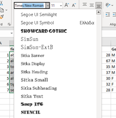
3. Click on the down arrow found above B, I, U. the default style is Calibri.

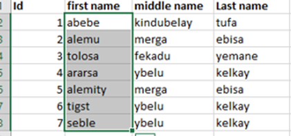
5. Finally, you will get the following result. Font style is changed from Calibri in to Times New Roman

Change Font size using Font formatting in Microsoft excel

You can change the font size of the text inside the excel document as follows.

1. Select the cell, rows, columns, or entire records.

2. Click on home menu.

3. Go to font tool.

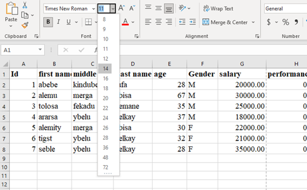
4. Click on the down arrow of the number found above B, I, U and right side of the font style. the default style is Calibri.

Text underline

You can add the line under the texts inside the excel document.

Steps

1. Select the cell, rows, columns, or entire records.

2. Click on home menu.

3. Go to font tool.

4. Click on the U latter. Or you can press CTRL + U from the keyboard.

Change Text color using Font formatting in Microsoft excel

You can change the color of texts in a single cell, columns, rows or entire records.

Steps

1. Select the cell, columns, rows or records you want to change the text color.
2. Click on home menu.
3. Go to font tool.
4. Click on the down arrow of A letter underlined by thick colored line as follows.

5. Click on the color you want.

Examples

1: change the color of single cell text.

2: change the color of single row text.

3: change the color of single column text.

Change text background color using Font formatting in Microsoft excel

You can change the background color of a single cell, columns, rows or the entire records.

Steps

1. Select the cell, columns, rows or records you want to change the text color.
2. Click on home menu.
3. Go to font tool.
4. Click on the down arrow of fill color icon underlined by thick colored line as follows. Then click on the color you want.

Examples

1: change background color for a single cell.

2: change background color for a single column.

3: change background color for records.

Text alignment

Using the alignment tool, you can align the cell, columns, rows, and records to the right, center or left. If the data inside the cell is text, the alignment is left by default. If the data is number, it is aligned to right by default. So, you can change the default alignment by following the following steps.

Steps

1. Select the cell, columns, rows, or records you are going to make align on it.

2. Click on home menu.

3. Go to alignment tool.

4. Click on the type of alignment you want to do.

Example 1: align column text center.

Text rotation (orientation)

You can rotate the texts inside a single cell, columns, rows, or the entire records diagonally or vertically.

Steps

1. Select the cell, columns, rows, or records you are going to make align on it.

2. Click on home menu.

3. Go to alignment tool.

4. Click on the down arrow of AB icon with diagonal arrow sign you want to do.

5. Select the type of rotation you want to apply.

Examples

1: rotate column text diagonal.

2: rotate the rows text vertical.

Wrap text

If you have long words or phrases in a single cell, some of the letter or word will be hidden or go beyond out of the cell. Because the length of cell is not much enough to accommodate all bodies of the text. The solution is wrapping the text, row cells, or column cells. This wrapping text makes the cell to show all word or letter.

1. Select the cell, column, or rows you need to wrap.
2. Click on home menu.
3. Go to alignment tool.
4. Click on the Wrap Text button.

Example: text in a cell go out of the border. After wrapping it, all the word is inside the cell.

Merge and center

In excel record, there may present main row and under main row there may present sub row. For column also may happen. This time you can make your main row or main column to cover more than one row or column respectively. Hence, merge and center is applicable for this situation.

Steps

1. Select the row cells or column cells you want to merge.
2. Click on home menu.
3. Go to alignment tool.
4. Click on the down arrow of Merge & Center button

5. Select the type merges

Example

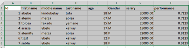
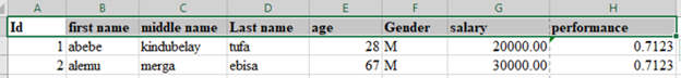
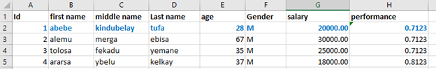
In the following record, the salary column has two sub column such as birr and cents. Hence, salary column should be merged & centered.

Hence, after merge & center, the salary column covers two columns as follows.

Add title or heading Microsoft excel

You may want to add general information for excel sheet. E.g., If the excel sheet has student assessment value, the excel will have school name, school director name, students’ section and other relevant information.

• The title or heading may need to cover more than one cell. No problem you can apply merge & center the rows or columns. For merge & center, refer the above section.

• You can also change many font formats such as font color, size, font style or make it bold.
• You can also change the background color of the header title.
• E.g., the above header title is changed to Time New Roman from font style, orange from font color and blue from background color.

Number styles using Font formatting in Microsoft excel

Excel has a tool that used to decide what type of numbers in a cell, rows, or columns should store. You can change the decimal numbers to fraction, decimal to currency number, decimal number to percentage or you may make the number as simply a text.

Steps

1. Select a cell, the row cells or column cells you want to change the number style.
2. Click on home menu.
3. Go to number tool.
4. Click on the down arrow of number option.

5. Select the type number.

Examples

1: general number

2: Percentile number

3: number in currency

To change the number to currency, in addition to the above procedure, click on the down arrow from the right side of dollar sign. You will get the following result.

Increase and decrease decimal digits

This tool enables you to increase and decrease the number of digits after the decimal point of real number.

Steps

1. Select a cell, the row cells or column cells you want to make change on the type of number.
2. Click on home menu.
3. Go to number tool.
4. Click on the backward and forward arrow icons if you want to increase the digits and decrease the digits respectively.

Examples

decrease the decimal digits after decimal point.

Before decreasing the number of digits after the decimal point.

After decreasing the number of digits by two decimal point.

thank you for reading.!!!. To know about our service visit https://info.ethioptec.com